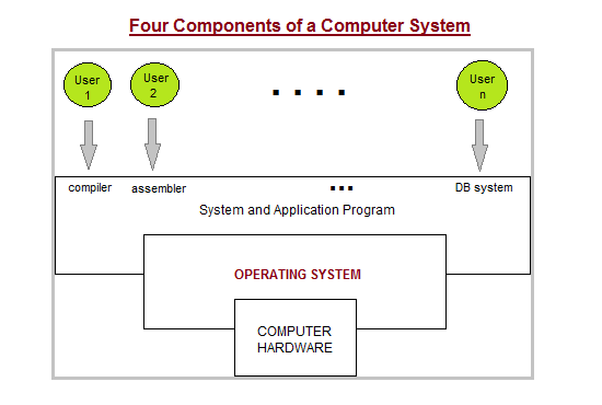
Introduction to Operating Systems

A computer system has many resources (hardware and software), which may be require to complete a task. The commonly required resources are input/output devices, memory, file storage space, CPU etc. The operating system acts as a manager of the above resources and allocates them to specific programs and users, whenever necessary to perform a particular task. Therefore operating system is the resource manager i.e. it can manage the resource of a computer system internally. The resources are processor, memory, files, and I/O devices. In simple terms, an operating system is the interface between the user and the machine.

Two Views of Operating System

User's View
System View

Operating System: User View

The user view of the computer refers to the interface being used. Such systems are designed for one user to monopolize its resources, to maximize the work that the user is performing. In these cases, the operating system is designed mostly for ease of use, with some attention paid to performance, and none paid to resource utilization.

Operating System: System View

Operating system can be viewed as a resource allocator also. A computer system consists of many resources like - hardware and software - that must be managed efficiently. The operating system acts as the manager of the resources, decides between conflicting requests, controls execution of programs etc.

Operating System Management Tasks

Processor management which involves putting the tasks into order and pairing them into manageable size before they go to the CPU.
Memory management which coordinates data to and from RAM (random-access memory) and determines the necessity for virtual memory.
Device management which provides interface between connected devices.
Storage management which directs permanent data storage.
Application which allows standard communication between software and your computer.
User interface which allows you to communicate with your computer.

Functions of Operating System

It boots the computer
It performs basic computer tasks e.g. managing the various peripheral devices e.g. mouse, keyboard
It provides a user interface, e.g. command line, graphical user interface (GUI)
It handles system resources such as computer's memory and sharing of the central processing unit(CPU) time by various applications or peripheral devices.
It provides file management which refers to the way that the operating system manipulates, stores, retrieves and saves data.
Error Handling is done by the operating system. It takes preventive measures whenever required to avoid errors.

Evolution of Operating Systems

The evolution of operating systems is directly dependent on the development of computer systems and how users use them. Here is a quick tour of computing systems through the past fifty years in the timeline.

Early Evolution

1945: ENIAC, Moore School of Engineering, University of Pennsylvania.
1949: EDSAC and EDVAC
1949: BINAC - a successor to the ENIAC
1951: UNIVAC by Remington
1952: IBM 701
1956: The interrupt
1954-1957: FORTRAN was developed

Operating Systems - Late 1950s

By the late 1950s Operating systems were well improved and started supporting following usages:

It was able to perform Single stream batch processing.
It could use Common, standardized, input/output routines for device access.
Program transition capabilities to reduce the overhead of starting a new job was added.
Error recovery to clean up after a job terminated abnormally was added.
Job control languages that allowed users to specify the job definition and resource requirements were made possible.

Operating Systems - In 1960s

1961: The dawn of minicomputers
1962: Compatible Time-Sharing System (CTSS) from MIT
1963: Burroughs Master Control Program (MCP) for the B5000 system
1964: IBM System/360
1960s: Disks became mainstream
1966: Minicomputers got cheaper, more powerful, and really useful.
1967-1968: Mouse was invented.
1964 and onward: Multics
1969: The UNIX Time-Sharing System from Bell Telephone Laboratories.

Supported OS Features by 1970s

Multi User and Multi tasking was introduced.
Dynamic address translation hardware and Virtual machines came into picture.
Modular architectures came into existence.
Personal, interactive systems came into existence.

Accomplishments after 1970

1971: Intel announces the microprocessor
1972: IBM comes out with VM: the Virtual Machine Operating System
1973: UNIX 4th Edition is published
1973: Ethernet
1974 The Personal Computer Age begins
1974: Gates and Allen wrote BASIC for the Altair
1976: Apple II
August 12, 1981: IBM introduces the IBM PC
1983 Microsoft begins work on MS-Windows
1984 Apple Macintosh comes out
1990 Microsoft Windows 3.0 comes out
1991 GNU/Linux
1992 The first Windows virus comes out
1993 Windows NT
2007: iOS
2008: Android OS

And as the research and development work continues, we are seeing new operating systems being developed and existing ones getting improved and modified to enhance the overall user experience, making operating systems fast and efficient like never before.

Also, with the onset of new devies like wearables, which includes, Smart Watches, Smart Glasses, VR gears etc, the demand for unconventional operating systems is also rising.

Types of Operating Systems

Following are some of the most widely used types of Operating system.

Simple Batch System
Multiprogramming Batch System
Multiprocessor System
Desktop System
Distributed Operating System
Clustered System
Realtime Operating System
Handheld System

Simple Batch Systems

In this type of system, there is no direct interaction between user and the computer.
The user has to submit a job (written on cards or tape) to a computer operator.
Then computer operator places a batch of several jobs on an input device.
Jobs are batched together by type of languages and requirement.
Then a special program, the monitor, manages the execution of each program in the batch.
The monitor is always in the main memory and available for execution.

Advantages of Simple Batch Systems

No interaction between user and computer.
No mechanism to prioritise the processes.

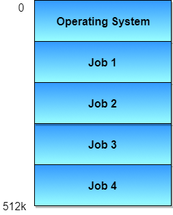
Multiprogramming Batch Systems

In this the operating system picks up and begins to execute one of the jobs from memory.
Once this job needs an I/O operation operating system switches to another job (CPU and OS always busy).
Jobs in the memory are always less than the number of jobs on disk(Job Pool).
If several jobs are ready to run at the same time, then the system chooses which one to run through the process of CPU Scheduling.
In Non-multiprogrammed system, there are moments when CPU sits idle and does not do any work.
In Multiprogramming system, CPU will never be idle and keeps on processing.

Time Sharing Systems are very similar to Multiprogramming batch systems. In fact time sharing systems are an extension of multiprogramming systems.

In Time sharing systems the prime focus is on minimizing the response time, while in multiprogramming the prime focus is to maximize the CPU usage.

Multiprocessor Systems

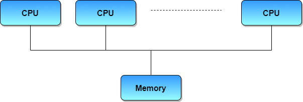
A Multiprocessor system consists of several processors that share a common physical memory. Multiprocessor system provides higher computing power and speed. In multiprocessor system all processors operate under single operating system. Multiplicity of the processors and how they do act together are transparent to the others.

Advantages of Multiprocessor Systems

Enhanced performance
Execution of several tasks by different processors concurrently, increases the system's throughput without speeding up the execution of a single task.
If possible, system divides task into many subtasks and then these subtasks can be executed in parallel in different processors. Thereby speeding up the execution of single tasks.

Desktop Systems

Earlier, CPUs and PCs lacked the features needed to protect an operating system from user programs. PC operating systems therefore were neither multiuser nor multitasking. However, the goals of these operating systems have changed with time; instead of maximizing CPU and peripheral utilization, the systems opt for maximizing user convenience and responsiveness. These systems are called Desktop Systems and include PCs running Microsoft Windows and the Apple Macintosh. Operating systems for these computers have benefited in several ways from the development of operating systems for mainframes.

Microcomputers were immediately able to adopt some of the technology developed for larger operating systems. On the other hand, the hardware costs for microcomputers are sufficiently low that individuals have sole use of the computer, and CPU utilization is no longer a prime concern. Thus, some of the design decisions made in operating systems for mainframes may not be appropriate for smaller systems.

Distributed Operating System

The motivation behind developing distributed operating systems is the availability of powerful and inexpensive microprocessors and advances in communication technology.

These advancements in technology have made it possible to design and develop distributed systems comprising of many computers that are inter connected by communication networks. The main benefit of distributed systems is its low price/performance ratio.

Advantages Distributed Operating System

As there are multiple systems involved, user at one site can utilize the resources of systems at other sites for resource-intensive tasks.
Fast processing.
Less load on the Host Machine.

Types of Distributed Operating Systems

Following are the two types of distributed operating systems used:

Client-Server Systems
Peer-to-Peer Systems

Client-Server Systems

Centralized systems today act as server systems to satisfy requests generated by client systems. The general structure of a client-server system is depicted in the figure below:

Server Systems can be broadly categorized as: Compute Servers and File Servers.

Compute Server systems, provide an interface to which clients can send requests to perform an action, in response to which they execute the action and send back results to the client.
File Server systems, provide a file-system interface where clients can create, update, read, and delete files.

Peer-to-Peer Systems

The growth of computer networks - especially the Internet and World Wide Web (WWW) – has had a profound influence on the recent development of operating systems. When PCs were introduced in the 1970s, they were designed for personal use and were generally considered standalone computers. With the beginning of widespread public use of the Internet in the 1990s for electronic mail and FTP, many PCs became connected to computer networks.

In contrast to the Tightly Coupled systems, the computer networks used in these applications consist of a collection of processors that do not share memory or a clock. Instead, each processor has its own local memory. The processors communicate with one another through various communication lines, such as high-speed buses or telephone lines. These systems are usually referred to as loosely coupled systems ( or distributed systems). The general structure of a client-server system is depicted in the figure below:

Clustered Systems

Like parallel systems, clustered systems gather together multiple CPUs to accomplish computational work.
Clustered systems differ from parallel systems, however, in that they are composed of two or more individual systems coupled together.
The definition of the term clustered is not concrete; the general accepted definition is that clustered computers share storage and are closely linked via LAN networking.
Clustering is usually performed to provide high availability.
A layer of cluster software runs on the cluster nodes. Each node can monitor one or more of the others. If the monitored machine fails, the monitoring machine can take ownership of its storage, and restart the application(s) that were running on the failed machine. The failed machine can remain down, but the users and clients of the application would only see a brief interruption of service.
Asymmetric Clustering - In this, one machine is in hot standby mode while the other is running the applications. The hot standby host (machine) does nothing but monitor the active server. If that server fails, the hot standby host becomes the active server.
Symmetric Clustering - In this, two or more hosts are running applications, and they are monitoring each other. This mode is obviously more efficient, as it uses all of the available hardware.
Parallel Clustering - Parallel clusters allow multiple hosts to access the same data on the shared storage. Because most operating systems lack support for this simultaneous data access by multiple hosts, parallel clusters are usually accomplished by special versions of software and special releases of applications.

Clustered technology is rapidly changing. Clustered system's usage and it's features should expand greatly as Storage Area Networks(SANs). SANs allow easy attachment of multiple hosts to multiple storage units. Current clusters are usually limited to two or four hosts due to the complexity of connecting the hosts to shared storage.

Real Time Operating System

It is defined as an operating system known to give maximum time for each of the critical operations that it performs, like OS calls and interrupt handling.

The Real-Time Operating system which guarantees the maximum time for critical operations and complete them on time are referred to as Hard Real-Time Operating Systems.

While the real-time operating systems that can only guarantee a maximum of the time, i.e. the critical task will get priority over other tasks, but no assurity of completeing it in a defined time. These systems are referred to as Soft Real-Time Operating Systems.

Handheld Systems

Handheld systems include Personal Digital Assistants(PDAs), such as Palm-Pilots or Cellular Telephones with connectivity to a network such as the Internet. They are usually of limited size due to which most handheld devices have a small amount of memory, include slow processors, and feature small display screens.

Many handheld devices have between 512 KB and 8 MB of memory. As a result, the operating system and applications must manage memory efficiently. This includes returning all allocated memory back to the memory manager once the memory is no longer being used.
Currently, many handheld devices do not use virtual memory techniques, thus forcing program developers to work within the confines of limited physical memory.
Processors for most handheld devices often run at a fraction of the speed of a processor in a PC. Faster processors require more power. To include a faster processor in a handheld device would require a larger battery that would have to be replaced more frequently.
The last issue confronting program designers for handheld devices is the small display screens typically available. One approach for displaying the content in web pages is web clipping, where only a small subset of a web page is delivered and displayed on the handheld device.

Some handheld devices may use wireless technology such as BlueTooth, allowing remote access to e-mail and web browsing. Cellular telephones with connectivity to the Internet fall into this category. Their use continues to expand as network connections become more available and other options such as cameras and MP3 players, expand their utility.

What is a Process?

A process is a program in execution. Process is not as same as program code but a lot more than it. A process is an 'active' entity as opposed to program which is considered to be a 'passive' entity. Attributes held by process include hardware state, memory, CPU etc.

Process memory is divided into four sections for efficient working :

The Text section is made up of the compiled program code, read in from non-volatile storage when the program is launched.
The Data section is made up the global and static variables, allocated and initialized prior to executing the main.
The Heap is used for the dynamic memory allocation, and is managed via calls to new, delete, malloc, free, etc.
The Stack is used for local variables. Space on the stack is reserved for local variables when they are declared.

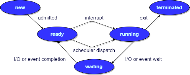
Different Process States

Processes in the operating system can be in any of the following states:

NEW- The process is being created.
READY- The process is waiting to be assigned to a processor.
RUNNING- Instructions are being executed.
WAITING- The process is waiting for some event to occur(such as an I/O completion or reception of a signal).
TERMINATED- The process has finished execution.

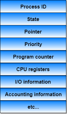
Process Control Block

There is a Process Control Block for each process, enclosing all the information about the process. It is a data structure, which contains the following:

Process State: It can be running, waiting etc.
Process ID and the parent process ID.
CPU registers and Program Counter. Program Counter holds the address of the next instruction to be executed for that process.
CPU Scheduling information: Such as priority information and pointers to scheduling queues.
Memory Management information: For example, page tables or segment tables.
Accounting information: The User and kernel CPU time consumed, account numbers, limits, etc.
I/O Status information: Devices allocated, open file tables, etc.

What is Process Scheduling?

The act of determining which process is in the ready state, and should be moved to the running state is known as Process Scheduling.

The prime aim of the process scheduling system is to keep the CPU busy all the time and to deliver minimum response time for all programs. For achieving this, the scheduler must apply appropriate rules for swapping processes IN and OUT of CPU.

Scheduling fell into one of the two general categories:

Non Pre-emptive Scheduling: When the currently executing process gives up the CPU voluntarily.
Pre-emptive Scheduling: When the operating system decides to favour another process, pre-empting the currently executing process.

What are Scheduling Queues?

All processes, upon entering into the system, are stored in the Job Queue.
Processes in the Ready state are placed in the Ready Queue.
Processes waiting for a device to become available are placed in Device Queues. There are unique device queues available for each I/O device.

A new process is initially put in the Ready queue. It waits in the ready queue until it is selected for execution(or dispatched). Once the process is assigned to the CPU and is executing, one of the following several events can occur:

The process could issue an I/O request, and then be placed in the I/O queue.
The process could create a new subprocess and wait for its termination.
The process could be removed forcibly from the CPU, as a result of an interrupt, and be put back in the ready queue.

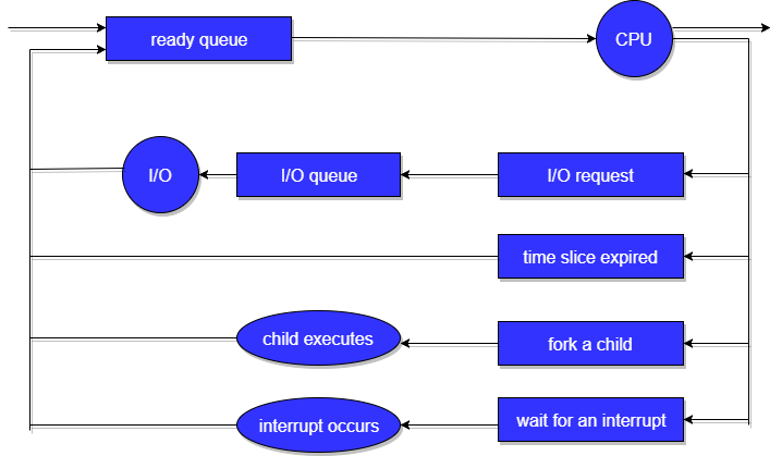
In the first two cases, the process eventually switches from the waiting state to the ready state, and is then put back in the ready queue. A process continues this cycle until it terminates, at which time it is removed from all queues and has its PCB and resources deallocated.

Types of Schedulers

There are three types of schedulers available:

Long Term Scheduler
Short Term Scheduler
Medium Term Scheduler

Let's discuss about all the different types of Schedulers in detail:

Long Term Scheduler

Long term scheduler runs less frequently. Long Term Schedulers decide which program must get into the job queue. From the job queue, the Job Processor, selects processes and loads them into the memory for execution. Primary aim of the Job Scheduler is to maintain a good degree of Multiprogramming. An optimal degree of Multiprogramming means the average rate of process creation is equal to the average departure rate of processes from the execution memory.

Short Term Scheduler

This is also known as CPU Scheduler and runs very frequently. The primary aim of this scheduler is to enhance CPU performance and increase process execution rate.

Medium Term Scheduler

This scheduler removes the processes from memory (and from active contention for the CPU), and thus reduces the degree of multiprogramming. At some later time, the process can be reintroduced into memory and its execution van be continued where it left off. This scheme is called swapping. The process is swapped out, and is later swapped in, by the medium term scheduler.

Swapping may be necessary to improve the process mix, or because a change in memory requirements has overcommitted available memory, requiring memory to be freed up. This complete process is descripted in the below diagram:

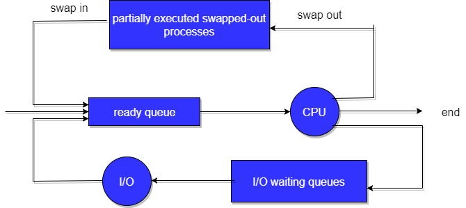
Addition of Medium-term scheduling to the queueing diagram.

What is Context Switch?

Switching the CPU to another process requires saving the state of the old process and loadingthe saved state for the new process. This task is known as a Context Switch.
The context of a process is represented in the Process Control Block(PCB) of a process; it includes the value of the CPU registers, the process state and memory-management information. When a context switch occurs, the Kernel saves the context of the old process in its PCB and loads the saved context of the new process scheduled to run.
Context switch time is pure overhead, because the system does no useful work while switching. Its speed varies from machine to machine, depending on the memory speed, the number of registers that must be copied, and the existence of special instructions(such as a single instruction to load or store all registers). Typical speeds range from 1 to 1000 microseconds.
Context Switching has become such a performance bottleneck that programmers are using new structures(threads) to avoid it whenever and wherever possible.

Operations on Process

Below we have discussed the two major operation Process Creation and Process Termination.

Process Creation

Through appropriate system calls, such as fork or spawn, processes may create other processes. The process which creates other process, is termed the parent of the other process, while the created sub-process is termed its child.

Each process is given an integer identifier, termed as process identifier, or PID. The parent PID (PPID) is also stored for each process.

On a typical UNIX systems the process scheduler is termed as sched, and is given PID 0. The first thing done by it at system start-up time is to launch init, which gives that process PID 1. Further Init launches all the system daemons and user logins, and becomes the ultimate parent of all other processes.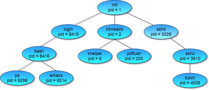

A child process may receive some amount of shared resources with its parent depending on system implementation. To prevent runaway children from consuming all of a certain system resource, child processes may or may not be limited to a subset of the resources originally allocated to the parent.

There are two options for the parent process after creating the child :

Wait for the child process to terminate before proceeding. Parent process makes a wait() system call, for either a specific child process or for any particular child process, which causes the parent process to block until the wait() returns. UNIX shells normally wait for their children to complete before issuing a new prompt.
Run concurrently with the child, continuing to process without waiting. When a UNIX shell runs a process as a background task, this is the operation seen. It is also possible for the parent to run for a while, and then wait for the child later, which might occur in a sort of a parallel processing operation.

There are also two possibilities in terms of the address space of the new process:

The child process is a duplicate of the parent process.
The child process has a program loaded into it.

To illustrate these different implementations, let us consider the UNIX operating system. In UNIX, each process is identified by its process identifier, which is a unique integer. A new process is created by the fork system call. The new process consists of a copy of the address space of the original process. This mechanism allows the parent process to communicate easily with its child process. Both processes (the parent and the child) continue execution at the instruction after the fork system call, with one difference: The return code for the fork system call is zero for the new(child) process, whereas the(non zero) process identifier of the child is returned to the parent.

Typically, the execlp system call is used after the fork system call by one of the two processes to replace the process memory space with a new program. The execlp system call loads a binary file into memory - destroying the memory image of the program containing the execlp system call – and starts its execution. In this manner the two processes are able to communicate, and then to go their separate ways.

Below is a C program to illustrate forking a separate process using UNIX(made using Ubuntu):

#include<stdio.h>

void main(int argc, char *argv[])
{
    int pid;

    /* Fork another process */
    pid = fork();

    if(pid < 0)
    {
        //Error occurred
        fprintf(stderr, "Fork Failed");
        exit(-1);
    }
    else if (pid == 0)
    {
        //Child process
        execlp("/bin/ls","ls",NULL);
    }
    else
    {
        //Parent process
        //Parent will wait for the child to complete
        wait(NULL);
        printf("Child complete");
        exit(0);
    }
}

GATE Numerical Tip: If fork is called for n times, the number of child processes or new processes created will be: 2n – 1.

Process Termination

By making the exit(system call), typically returning an int, processes may request their own termination. This int is passed along to the parent if it is doing a wait(), and is typically zero on successful completion and some non-zero code in the event of any problem.

Processes may also be terminated by the system for a variety of reasons, including :

The inability of the system to deliver the necessary system resources.
In response to a KILL command or other unhandled process interrupts.
A parent may kill its children if the task assigned to them is no longer needed i.e. if the need of having a child terminates.
If the parent exits, the system may or may not allow the child to continue without a parent (In UNIX systems, orphaned processes are generally inherited by init, which then proceeds to kill them.)

When a process ends, all of its system resources are freed up, open files flushed and closed, etc. The process termination status and execution times are returned to the parent if the parent is waiting for the child to terminate, or eventually returned to init if the process already became an orphan.

The processes which are trying to terminate but cannot do so because their parent is not waiting for them are termed zombies. These are eventually inherited by init as orphans and killed off.

What is CPU Scheduling?

CPU scheduling is a process which allows one process to use the CPU while the execution of another process is on hold(in waiting state) due to unavailability of any resource like I/O etc, thereby making full use of CPU. The aim of CPU scheduling is to make the system efficient, fast and fair.

Whenever the CPU becomes idle, the operating system must select one of the processes in the ready queue to be executed. The selection process is carried out by the short-term scheduler (or CPU scheduler). The scheduler selects from among the processes in memory that are ready to execute, and allocates the CPU to one of them.

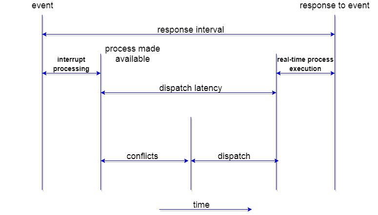
CPU Scheduling: Dispatcher

Another component involved in the CPU scheduling function is the Dispatcher. The dispatcher is the module that gives control of the CPU to the process selected by the short-term scheduler. This function involves:

Switching context
Switching to user mode
Jumping to the proper location in the user program to restart that program from where it left last time.

The dispatcher should be as fast as possible, given that it is invoked during every process switch. The time taken by the dispatcher to stop one process and start another process is known as the Dispatch Latency. Dispatch Latency can be explained using the below figure:

Types of CPU Scheduling

CPU scheduling decisions may take place under the following four circumstances:

When a process switches from the running state to the waiting state(for I/O request or invocation of wait for the termination of one of the child processes).
When a process switches from the running state to the ready state (for example, when an interrupt occurs).
When a process switches from the waiting state to the ready state(for example, completion of I/O).
When a process terminates.

In circumstances 1 and 4, there is no choice in terms of scheduling. A new process(if one exists in the ready queue) must be selected for execution. There is a choice, however in circumstances 2 and 3.

When Scheduling takes place only under circumstances 1 and 4, we say the scheduling scheme is non-preemptive; otherwise the scheduling scheme is preemptive.

Non-Preemptive Scheduling

Under non-preemptive scheduling, once the CPU has been allocated to a process, the process keeps the CPU until it releases the CPU either by terminating or by switching to the waiting state.

This scheduling method is used by the Microsoft Windows 3.1 and by the Apple Macintosh operating systems.

It is the only method that can be used on certain hardware platforms, because It does not require the special hardware(for example: a timer) needed for preemptive scheduling.

Preemptive Scheduling

In this type of Scheduling, the tasks are usually assigned with priorities. At times it is necessary to run a certain task that has a higher priority before another task although it is running. Therefore, the running task is interrupted for some time and resumed later when the priority task has finished its execution.

CPU Scheduling: Scheduling Criteria

There are many different criterias to check when considering the "best" scheduling algorithm, they are:

CPU Utilization

To make out the best use of CPU and not to waste any CPU cycle, CPU would be working most of the time(Ideally 100% of the time). Considering a real system, CPU usage should range from 40% (lightly loaded) to 90% (heavily loaded.)

Throughput

It is the total number of processes completed per unit time or rather say total amount of work done in a unit of time. This may range from 10/second to 1/hour depending on the specific processes.

Turnaround Time

It is the amount of time taken to execute a particular process, i.e. The interval from time of submission of the process to the time of completion of the process(Wall clock time).

Waiting Time

The sum of the periods spent waiting in the ready queue amount of time a process has been waiting in the ready queue to acquire get control on the CPU.

Load Average

It is the average number of processes residing in the ready queue waiting for their turn to get into the CPU.

Response Time

Amount of time it takes from when a request was submitted until the first response is produced. Remember, it is the time till the first response and not the completion of process execution(final response).

In general CPU utilization and Throughput are maximized and other factors are reduced for proper optimization.

Scheduling Algorithms

To decide which process to execute first and which process to execute last to achieve maximum CPU utilisation, computer scientists have defined some algorithms, they are:

First Come First Serve(FCFS) Scheduling
Shortest-Job-First(SJF) Scheduling
Priority Scheduling
Round Robin(RR) Scheduling
Multilevel Queue Scheduling
Multilevel Feedback Queue Scheduling

We will be discussing all the scheduling algorithms, one by one, in detail in the next tutorials.

First Come First Serve Scheduling

In the "First come first serve" scheduling algorithm, as the name suggests, the process which arrives first, gets executed first, or we can say that the process which requests the CPU first, gets the CPU allocated first.

First Come First Serve, is just like FIFO(First in First out) Queue data structure, where the data element which is added to the queue first, is the one who leaves the queue first.
This is used in Batch Systems.
It's easy to understand and implement programmatically, using a Queue data structure, where a new process enters through the tail of the queue, and the scheduler selects process from the head of the queue.
A perfect real life example of FCFS scheduling is buying tickets at ticket counter.

Calculating Average Waiting Time

For every scheduling algorithm, Average waiting time is a crucial parameter to judge it's performance.

AWT or Average waiting time is the average of the waiting times of the processes in the queue, waiting for the scheduler to pick them for execution.

Lower the Average Waiting Time, better the scheduling algorithm.

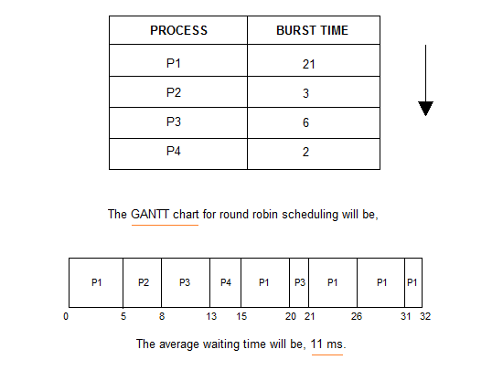
Consider the processes P1, P2, P3, P4 given in the below table, arrives for execution in the same order, with Arrival Time 0, and given Burst Time, let's find the average waiting time using the FCFS scheduling algorithm.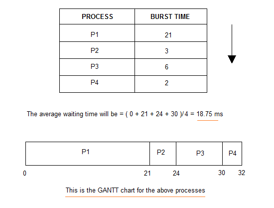

The average waiting time will be 18.75 ms

For the above given proccesses, first P1 will be provided with the CPU resources,

Hence, waiting time for P1 will be 0
P1 requires 21 ms for completion, hence waiting time for P2 will be 21 ms
Similarly, waiting time for process P3 will be execution time of P1 + execution time for P2, which will be (21 + 3) ms = 24 ms.
For process P4 it will be the sum of execution times of P1, P2 and P3.

The GANTT chart above perfectly represents the waiting time for each process.

Problems with FCFS Scheduling

Below we have a few shortcomings or problems with the FCFS scheduling algorithm:

It is Non Pre-emptive algorithm, which means the process priority doesn't matter.
If a process with very least priority is being executed, more like daily routine backup process, which takes more time, and all of a sudden some other high priority process arrives, like interrupt to avoid system crash, the high priority process will have to wait, and hence in this case, the system will crash, just because of improper process scheduling.
Not optimal Average Waiting Time.
Resources utilization in parallel is not possible, which leads to Convoy Effect, and hence poor resource(CPU, I/O etc) utilization.

What is Convoy Effect?

Convoy Effect is a situation where many processes, who need to use a resource for short time are blocked by one process holding that resource for a long time.

This essentially leads to poort utilization of resources and hence poor performance.

Program for FCFS Scheduling

Here we have a simple C++ program for processes with arrival time as 0.

In the program, we will be calculating the Average waiting time and Average turn around time for a given array of Burst times for the list of processes.

/* Simple C++ program for implementation 
of FCFS scheduling */

#include<iostream>

using namespace std;
 
// function to find the waiting time for all processes
void findWaitingTime(int processes[], int n, int bt[], int wt[])
{
    // waiting time for first process will be 0
    wt[0] = 0;
 
    // calculating waiting time
    for (int i = 1; i < n ; i++)
    {
        wt[i] =  bt[i-1] + wt[i-1];
    }
}
 
// function to calculate turn around time
void findTurnAroundTime( int processes[], int n, int bt[], int wt[], int tat[])
{
    // calculating turnaround time by adding
    // bt[i] + wt[i]
    for (int i = 0; i < n ; i++)
    {
        tat[i] = bt[i] + wt[i];
    }
}
 
// function to calculate average time
void findAverageTime( int processes[], int n, int bt[])
{
    int wt[n], tat[n], total_wt = 0, total_tat = 0;
 
    // function to find waiting time of all processes
    findWaitingTime(processes, n, bt, wt);
 
    // function to find turn around time for all processes
    findTurnAroundTime(processes, n, bt, wt, tat);
 
    // display processes along with all details
    cout << "Processes  "<< " Burst time  "<< " Waiting time  " << " Turn around time\n";
 
    // calculate total waiting time and total turn around time
    for (int i = 0; i < n; i++)
    {
        total_wt = total_wt + wt[i];
        total_tat = total_tat + tat[i];
        cout << "   " << i+1 << "\t\t" << bt[i] <<"\t    "<< wt[i] <<"\t\t  " << tat[i] <<endl;
    }
 
    cout << "Average waiting time = "<< (float)total_wt / (float)n;
    cout << "\nAverage turn around time = "<< (float)total_tat / (float)n;
}
 
// main function
int main()
{
    // process ids
    int processes[] = { 1, 2, 3, 4};
    int n = sizeof processes / sizeof processes[0];
 
    // burst time of all processes
    int  burst_time[] = {21, 3, 6, 2};
 
    findAverageTime(processes, n,  burst_time);
    
    return 0;
}

Processes Burst time Waiting time Turn around time
1 21 0 21
2 3 21 24
3 6 24 30
4 2 30 32
Average waiting time = 18.75
Average turn around time = 26.75

Here we have simple formulae for calculating various times for given processes:

Completion Time: Time taken for the execution to complete, starting from arrival time.

Turn Around Time: Time taken to complete after arrival. In simple words, it is the difference between the Completion time and the Arrival time.

Waiting Time: Total time the process has to wait before it's execution begins. It is the difference between the Turn Around time and the Burst time of the process.

For the program above, we have considered the arrival time to be 0 for all the processes, try to implement a program with variable arrival times.

Shortest Job First(SJF) Scheduling

Shortest Job First scheduling works on the process with the shortest burst time or duration first.

This is the best approach to minimize waiting time.
This is used in Batch Systems.
It is of two types:
1. Non Pre-emptive
2. Pre-emptive
To successfully implement it, the burst time/duration time of the processes should be known to the processor in advance, which is practically not feasible all the time.
This scheduling algorithm is optimal if all the jobs/processes are available at the same time. (either Arrival time is 0 for all, or Arrival time is same for all)

Non Pre-emptive Shortest Job First

Consider the below processes available in the ready queue for execution, with arrival time as 0 for all and given burst times.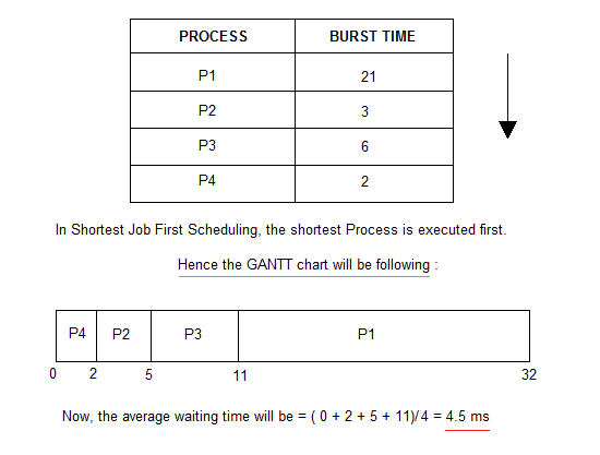

As you can see in the GANTT chart above, the process P4 will be picked up first as it has the shortest burst time, then P2, followed by P3 and at last P1.

We scheduled the same set of processes using the First come first serve algorithm in the previous tutorial, and got average waiting time to be 18.75 ms, whereas with SJF, the average waiting time comes out 4.5 ms.

Problem with Non Pre-emptive SJF

If the arrival time for processes are different, which means all the processes are not available in the ready queue at time 0, and some jobs arrive after some time, in such situation, sometimes process with short burst time have to wait for the current process's execution to finish, because in Non Pre-emptive SJF, on arrival of a process with short duration, the existing job/process's execution is not halted/stopped to execute the short job first.

This leads to the problem of Starvation, where a shorter process has to wait for a long time until the current longer process gets executed. This happens if shorter jobs keep coming, but this can be solved using the concept of aging.

Pre-emptive Shortest Job First

In Preemptive Shortest Job First Scheduling, jobs are put into ready queue as they arrive, but as a process with short burst time arrives, the existing process is preempted or removed from execution, and the shorter job is executed first.

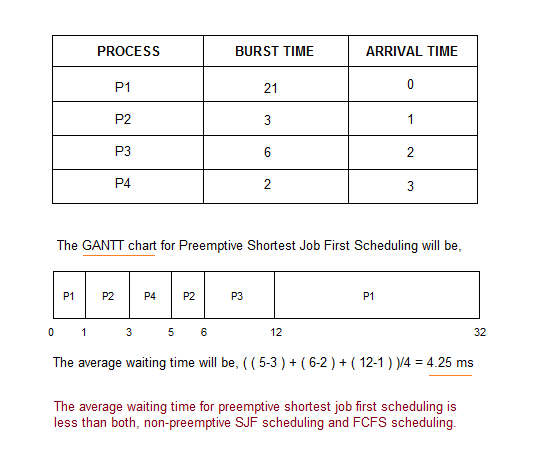
As you can see in the GANTT chart above, as P1 arrives first, hence it's execution starts immediately, but just after 1 ms, process P2 arrives with a burst time of 3 ms which is less than the burst time of P1, hence the process P1(1 ms done, 20 ms left) is preemptied and process P2 is executed.

As P2 is getting executed, after 1 ms, P3 arrives, but it has a burst time greater than that of P2, hence execution of P2 continues. But after another millisecond, P4 arrives with a burst time of 2 ms, as a result P2(2 ms done, 1 ms left) is preemptied and P4 is executed.

After the completion of P4, process P2 is picked up and finishes, then P2 will get executed and at last P1.

The Pre-emptive SJF is also known as Shortest Remaining Time First, because at any given point of time, the job with the shortest remaining time is executed first.

Program for SJF Scheduling

In the below program, we consider the arrival time of all the jobs to be 0.

Also, in the program, we will sort all the jobs based on their burst time and then execute them one by one, just like we did in FCFS scheduling program.

// c++ program to implement Shortest Job first

#include<bits/stdc++.h>

using namespace std;
 
struct Process
{
   int pid;     // process ID
   int bt;      // burst Time
};
 
/* 
    this function is used for sorting all
    processes in increasing order of burst time
*/
bool comparison(Process a, Process b)
{
    return (a.bt < b.bt);
}
 
// function to find the waiting time for all processes
void findWaitingTime(Process proc[], int n, int wt[])
{
    // waiting time for first process is 0
    wt[0] = 0;
 
    // calculating waiting time
    for (int i = 1; i < n ; i++)
    {
        wt[i] = proc[i-1].bt + wt[i-1] ;
    }
}
 
// function to calculate turn around time
void findTurnAroundTime(Process proc[], int n, int wt[], int tat[])
{
    // calculating turnaround time by adding bt[i] + wt[i]
    for (int i = 0; i < n ; i++)
    {
        tat[i] = proc[i].bt + wt[i];
    }
}
 
// function to calculate average time
void findAverageTime(Process proc[], int n)
{
    int wt[n], tat[n], total_wt = 0, total_tat = 0;
 
    // function to find waiting time of all processes
    findWaitingTime(proc, n, wt);
 
    // function to find turn around time for all processes
    findTurnAroundTime(proc, n, wt, tat);
 
    // display processes along with all details
    cout << "\nProcesses "<< " Burst time "
         << " Waiting time " << " Turn around time\n";
 
    // calculate total waiting time and total turn around time
    for (int i = 0; i < n; i++)
    {
        total_wt = total_wt + wt[i];
        total_tat = total_tat + tat[i];
        cout << " " << proc[i].pid << "\t\t"
             << proc[i].bt << "\t " << wt[i]
             << "\t\t " << tat[i] <<endl;
    }
 
    cout << "Average waiting time = "
         << (float)total_wt / (float)n;
    cout << "\nAverage turn around time = "
         << (float)total_tat / (float)n;
}
 
// main function
int main()
{
    Process proc[] = {{1, 21}, {2, 3}, {3, 6}, {4, 2}};
    int n = sizeof proc / sizeof proc[0];
 
    // sorting processes by burst time.
    sort(proc, proc + n, comparison);
 
    cout << "Order in which process gets executed\n";
    for (int i = 0 ; i < n; i++)
    {
        cout << proc[i].pid <<" ";
    }
 
    findAverageTime(proc, n);
    
    return 0;
}

Order in which process gets executed
4 2 3 1
Processes Burst time Waiting time Turn around time
4 2 0 2
2 3 2 5
3 6 5 11
1 21 11 32
Average waiting time = 4.5
Average turn around time = 12.5

Try implementing the program for SJF with variable arrival time for different jobs, yourself.

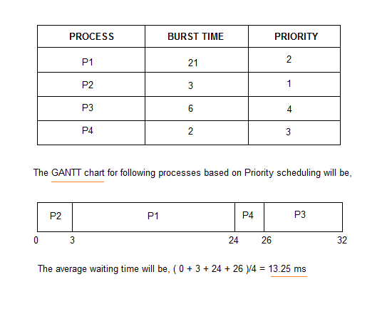
Priority Scheduling

Priority is assigned for each process.
Process with highest priority is executed first and so on.
Processes with same priority are executed in FCFS manner.
Priority can be decided based on memory requirements, time requirements or any other resource requirement.

Round Robin Scheduling

A fixed time is allotted to each process, called quantum, for execution.
Once a process is executed for given time period that process is preemptied and other process executes for given time period.
Context switching is used to save states of preemptied processes.

Multilevel Queue Scheduling

Another class of scheduling algorithms has been created for situations in which processes are easily classified into different groups.

For example: A common division is made between foreground(or interactive) processes and background (or batch) processes. These two types of processes have different response-time requirements, and so might have different scheduling needs. In addition, foreground processes may have priority over background processes.

A multi-level queue scheduling algorithm partitions the ready queue into several separate queues. The processes are permanently assigned to one queue, generally based on some property of the process, such as memory size, process priority, or process type. Each queue has its own scheduling algorithm.

For example: separate queues might be used for foreground and background processes. The foreground queue might be scheduled by Round Robin algorithm, while the background queue is scheduled by an FCFS algorithm.

In addition, there must be scheduling among the queues, which is commonly implemented as fixed-priority preemptive scheduling. For example: The foreground queue may have absolute priority over the background queue.

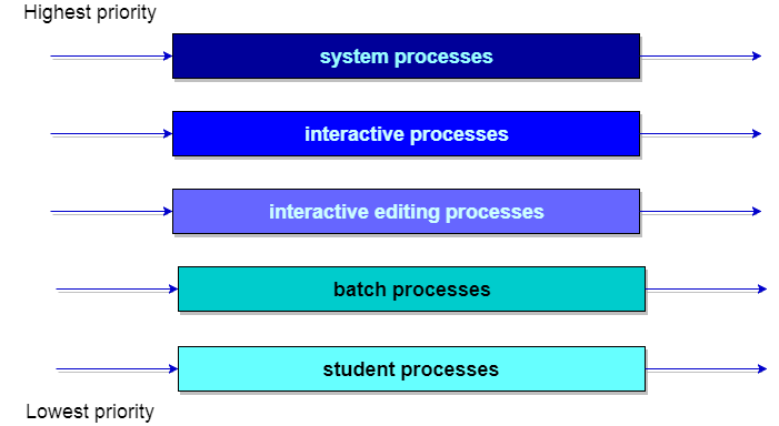
Let us consider an example of a multilevel queue-scheduling algorithm with five queues:

System Processes
Interactive Processes
Interactive Editing Processes
Batch Processes
Student Processes

Each queue has absolute priority over lower-priority queues. No process in the batch queue, for example, could run unless the queues for system processes, interactive processes, and interactive editing processes were all empty. If an interactive editing process entered the ready queue while a batch process was running, the batch process will be preempted.

Multilevel Feedback Queue Scheduling

In a multilevel queue-scheduling algorithm, processes are permanently assigned to a queue on entry to the system. Processes do not move between queues. This setup has the advantage of low scheduling overhead, but the disadvantage of being inflexible.

Multilevel feedback queue scheduling, however, allows a process to move between queues. The idea is to separate processes with different CPU-burst characteristics. If a process uses too much CPU time, it will be moved to a lower-priority queue. Similarly, a process that waits too long in a lower-priority queue may be moved to a higher-priority queue. This form of aging prevents starvation.

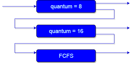
An example of a multilevel feedback queue can be seen in the below figure.

In general, a multilevel feedback queue scheduler is defined by the following parameters:

The number of queues.
The scheduling algorithm for each queue.
The method used to determine when to upgrade a process to a higher-priority queue.
The method used to determine when to demote a process to a lower-priority queue.
The method used to determine which queue a process will enter when that process needs service.

The definition of a multilevel feedback queue scheduler makes it the most general CPU-scheduling algorithm. It can be configured to match a specific system under design. Unfortunately, it also requires some means of selecting values for all the parameters to define the best scheduler. Although a multilevel feedback queue is the most general scheme, it is also the most complex.

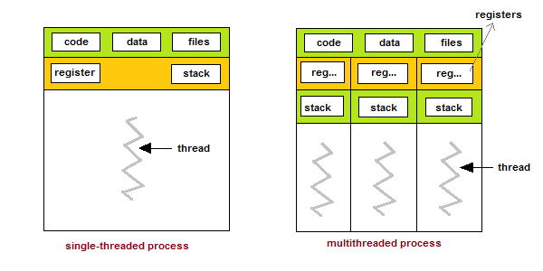
What are Threads?

Thread is an execution unit which consists of its own program counter, a stack, and a set of registers. Threads are also known as Lightweight processes. Threads are popular way to improve application through parallelism. The CPU switches rapidly back and forth among the threads giving illusion that the threads are running in parallel.

As each thread has its own independent resource for process execution, multpile processes can be executed parallely by increasing number of threads.

Single Threaded and Multithreaded Process

Types of Thread

There are two types of threads:

User Threads
Kernel Threads

User threads, are above the kernel and without kernel support. These are the threads that application programmers use in their programs.

Kernel threads are supported within the kernel of the OS itself. All modern OSs support kernel level threads, allowing the kernel to perform multiple simultaneous tasks and/or to service multiple kernel system calls simultaneously.

Multithreading Models

The user threads must be mapped to kernel threads, by one of the following strategies:

Many to One Model
One to One Model
Many to Many Model

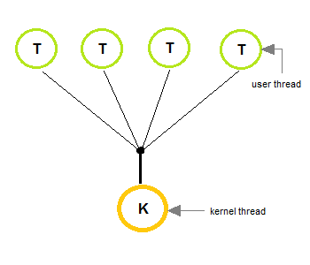
Many to One Model

In the many to one model, many user-level threads are all mapped onto a single kernel thread.
Thread management is handled by the thread library in user space, which is efficient in nature.

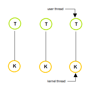
One to One Model

The one to one model creates a separate kernel thread to handle each and every user thread.
Most implementations of this model place a limit on how many threads can be created.
Linux and Windows from 95 to XP implement the one-to-one model for threads.

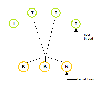
Many to Many Model

The many to many model multiplexes any number of user threads onto an equal or smaller number of kernel threads, combining the best features of the one-to-one and many-to-one models.
Users can create any number of the threads.
Blocking the kernel system calls does not block the entire process.
Processes can be split across multiple processors.

What are Thread Libraries?

Thread libraries provide programmers with API for creation and management of threads.

Thread libraries may be implemented either in user space or in kernel space. The user space involves API functions implemented solely within the user space, with no kernel support. The kernel space involves system calls, and requires a kernel with thread library support.

Three types of Thread

POSIX Pitheads, may be provided as either a user or kernel library, as an extension to the POSIX standard.
Win32 threads, are provided as a kernel-level library on Windows systems.
Java threads: Since Java generally runs on a Java Virtual Machine, the implementation of threads is based upon whatever OS and hardware the JVM is running on, i.e. either Pitheads or Win32 threads depending on the system.

Benefits of Multithreading

Responsiveness
Resource sharing, hence allowing better utilization of resources.
Economy. Creating and managing threads becomes easier.
Scalability. One thread runs on one CPU. In Multithreaded processes, threads can be distributed over a series of processors to scale.
Context Switching is smooth. Context switching refers to the procedure followed by CPU to change from one task to another.

Multithreading Issues

Below we have mentioned a few issues related to multithreading. Well, it's an old saying, All good things, come at a price.

Thread Cancellation

Thread cancellation means terminating a thread before it has finished working. There can be two approaches for this, one is Asynchronous cancellation, which terminates the target thread immediately. The other is Deferred cancellation allows the target thread to periodically check if it should be cancelled.

Signal Handling

Signals are used in UNIX systems to notify a process that a particular event has occurred. Now in when a Multithreaded process receives a signal, to which thread it must be delivered? It can be delivered to all, or a single thread.

fork() System Call

fork() is a system call executed in the kernel through which a process creates a copy of itself. Now the problem in Multithreaded process is, if one thread forks, will the entire process be copied or not?

Security Issues

Yes, there can be security issues because of extensive sharing of resources between multiple threads.

There are many other issues that you might face in a multithreaded process, but there are appropriate solutions available for them. Pointing out some issues here was just to study both sides of the coin.

Process Synchronization

Process Synchronization means sharing system resources by processes in a such a way that, Concurrent access to shared data is handled thereby minimizing the chance of inconsistent data. Maintaining data consistency demands mechanisms to ensure synchronized execution of cooperating processes.

Process Synchronization was introduced to handle problems that arose while multiple process executions. Some of the problems are discussed below.

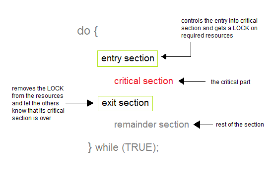
Critical Section Problem

A Critical Section is a code segment that accesses shared variables and has to be executed as an atomic action. It means that in a group of cooperating processes, at a given point of time, only one process must be executing its critical section. If any other process also wants to execute its critical section, it must wait until the first one finishes.

Solution to Critical Section Problem

A solution to the critical section problem must satisfy the following three conditions:

1. Mutual Exclusion

Out of a group of cooperating processes, only one process can be in its critical section at a given point of time.

2. Progress

If no process is in its critical section, and if one or more threads want to execute their critical section then any one of these threads must be allowed to get into its critical section.

3. Bounded Waiting

After a process makes a request for getting into its critical section, there is a limit for how many other processes can get into their critical section, before this process's request is granted. So after the limit is reached, system must grant the process permission to get into its critical section.

Synchronization Hardware

Many systems provide hardware support for critical section code. The critical section problem could be solved easily in a single-processor environment if we could disallow interrupts to occur while a shared variable or resource is being modified.

In this manner, we could be sure that the current sequence of instructions would be allowed to execute in order without pre-emption. Unfortunately, this solution is not feasible in a multiprocessor environment.

Disabling interrupt on a multiprocessor environment can be time consuming as the message is passed to all the processors.

This message transmission lag, delays entry of threads into critical section and the system efficiency decreases.

Mutex Locks

As the synchronization hardware solution is not easy to implement for everyone, a strict software approach called Mutex Locks was introduced. In this approach, in the entry section of code, a LOCK is acquired over the critical resources modified and used inside critical section, and in the exit section that LOCK is released.

As the resource is locked while a process executes its critical section hence no other process can access it.

Introduction to Semaphores

In 1965, Dijkstra proposed a new and very significant technique for managing concurrent processes by using the value of a simple integer variable to synchronize the progress of interacting processes. This integer variable is called semaphore. So it is basically a synchronizing tool and is accessed only through two low standard atomic operations, wait and signal designated by P(S) and V(S)respectively.

In very simple words, semaphore is a variable which can hold only a non-negative Integer value, shared between all the threads, with operations wait and signal, which work as follow:

P(S): if S ≥ 1 then S := S - 1
      else <block and enqueue the process>;

V(S): if <some process is blocked on the queue>
        then <unblock a process>
      else S := S + 1;

The classical definitions of wait and signal are:

Wait: Decrements the value of its argument S, as soon as it would become non-negative(greater than or equal to 1).
Signal: Increments the value of its argument S, as there is no more process blocked on the queue.

Properties of Semaphores

It's simple and always have a non-negative Integer value.
Works with many processes.
Can have many different critical sections with different semaphores.
Each critical section has unique access semaphores.
Can permit multiple processes into the critical section at once, if desirable.

Types of Semaphores

Semaphores are mainly of two types:

Binary Semaphore:
It is a special form of semaphore used for implementing mutual exclusion, hence it is often called a Mutex. A binary semaphore is initialized to 1 and only takes the values 0 and 1 during execution of a program.
Counting Semaphores:
These are used to implement bounded concurrency.

Example of Use

Here is a simple step wise implementation involving declaration and usage of semaphore.

Shared var mutex: semaphore = 1;
Process i
    begin
    .
    .
    P(mutex);
    execute CS;
    V(mutex);
    .
    .
    End;

Limitations of Semaphores

Priority Inversion is a big limitation of semaphores.
Their use is not enforced, but is by convention only.
With improper use, a process may block indefinitely. Such a situation is called Deadlock. We will be studying deadlocks in details in coming lessons.

Classical Problems of Synchronization

In this tutorial we will discuss about various classic problem of synchronization.

Semaphore can be used in other synchronization problems besides Mutual Exclusion.

Below are some of the classical problem depicting flaws of process synchronaization in systems where cooperating processes are present.

We will discuss the following three problems:

Bounded Buffer (Producer-Consumer) Problem
The Readers Writers Problem
Dining Philosophers Problem

Bounded Buffer Problem

This problem is generalised in terms of the Producer Consumer problem, where a finite buffer pool is used to exchange messages between producer and consumer processes.

Because the buffer pool has a maximum size, this problem is often called the Bounded buffer problem.

Solution to this problem is, creating two counting semaphores "full" and "empty" to keep track of the current number of full and empty buffers respectively.

The Readers Writers Problem

In this problem there are some processes(called readers) that only read the shared data, and never change it, and there are other processes(called writers) who may change the data in addition to reading, or instead of reading it.
There are various type of readers-writers problem, most centred on relative priorities of readers and writers.

Dining Philosophers Problem

The dining philosopher's problem involves the allocation of limited resources to a group of processes in a deadlock-free and starvation-free manner.
There are five philosophers sitting around a table, in which there are five chopsticks/forks kept beside them and a bowl of rice in the centre, When a philosopher wants to eat, he uses two chopsticks - one from their left and one from their right. When a philosopher wants to think, he keeps down both chopsticks at their original place.

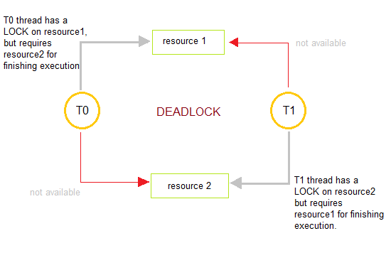
What is a Deadlock?

Deadlocks are a set of blocked processes each holding a resource and waiting to acquire a resource held by another process.

How to avoid Deadlocks

Deadlocks can be avoided by avoiding at least one of the four conditions, because all this four conditions are required simultaneously to cause deadlock.

Mutual Exclusion
Resources shared such as read-only files do not lead to deadlocks but resources, such as printers and tape drives, requires exclusive access by a single process.
Hold and Wait
In this condition processes must be prevented from holding one or more resources while simultaneously waiting for one or more others.
No Preemption
Preemption of process resource allocations can avoid the condition of deadlocks, where ever possible.
Circular Wait
Circular wait can be avoided if we number all resources, and require that processes request resources only in strictly increasing(or decreasing) order.

Handling Deadlock

The above points focus on preventing deadlocks. But what to do once a deadlock has occured. Following three strategies can be used to remove deadlock after its occurrence.

Preemption
We can take a resource from one process and give it to other. This will resolve the deadlock situation, but sometimes it does causes problems.
Rollback
In situations where deadlock is a real possibility, the system can periodically make a record of the state of each process and when deadlock occurs, roll everything back to the last checkpoint, and restart, but allocating resources differently so that deadlock does not occur.
Kill one or more processes
This is the simplest way, but it works.

What is a Livelock?

There is a variant of deadlock called livelock. This is a situation in which two or more processes continuously change their state in response to changes in the other process(es) without doing any useful work. This is similar to deadlock in that no progress is made but differs in that neither process is blocked or waiting for anything.

A human example of livelock would be two people who meet face-to-face in a corridor and each moves aside to let the other pass, but they end up swaying from side to side without making any progress because they always move the same way at the same time.

Introduction to Memory Management

Main Memory refers to a physical memory that is the internal memory to the computer. The word main is used to distinguish it from external mass storage devices such as disk drives. Main memory is also known as RAM. The computer is able to change only data that is in main memory. Therefore, every program we execute and every file we access must be copied from a storage device into main memory.

All the programs are loaded in the main memeory for execution. Sometimes complete program is loaded into the memory, but some times a certain part or routine of the program is loaded into the main memory only when it is called by the program, this mechanism is called Dynamic Loading, this enhance the performance.

Also, at times one program is dependent on some other program. In such a case, rather than loading all the dependent programs, CPU links the dependent programs to the main executing program when its required. This mechanism is known as Dynamic Linking.

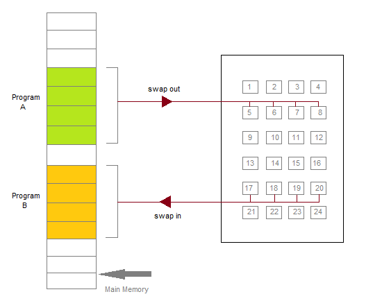
Swapping

A process needs to be in memory for execution. But sometimes there is not enough main memory to hold all the currently active processes in a timesharing system. So, excess process are kept on disk and brought in to run dynamically. Swapping is the process of bringing in each process in main memory, running it for a while and then putting it back to the disk.

Contiguous Memory Allocation

In contiguous memory allocation each process is contained in a single contiguous block of memory. Memory is divided into several fixed size partitions. Each partition contains exactly one process. When a partition is free, a process is selected from the input queue and loaded into it. The free blocks of memory are known as holes. The set of holes is searched to determine which hole is best to allocate.

Memory Protection

Memory protection is a phenomenon by which we control memory access rights on a computer. The main aim of it is to prevent a process from accessing memory that has not been allocated to it. Hence prevents a bug within a process from affecting other processes, or the operating system itself, and instead results in a segmentation fault or storage violation exception being sent to the disturbing process, generally killing of process.

Memory Allocation

Memory allocation is a process by which computer programs are assigned memory or space. It is of three types :

First Fit:
The first hole that is big enough is allocated to program.
Best Fit:
The smallest hole that is big enough is allocated to program.
Worst Fit:
The largest hole that is big enough is allocated to program.

Fragmentation

Fragmentation occurs in a dynamic memory allocation system when most of the free blocks are too small to satisfy any request. It is generally termed as inability to use the available memory.

In such situation processes are loaded and removed from the memory. As a result of this, free holes exists to satisfy a request but is non contiguous i.e. the memory is fragmented into large no. Of small holes. This phenomenon is known as External Fragmentation.

Also, at times the physical memory is broken into fixed size blocks and memory is allocated in unit of block sizes. The memory allocated to a space may be slightly larger than the requested memory. The difference between allocated and required memory is known as Internal fragmentation i.e. the memory that is internal to a partition but is of no use.

Paging

A solution to fragmentation problem is Paging. Paging is a memory management mechanism that allows the physical address space of a process to be non-contagious. Here physical memory is divided into blocks of equal size called Pages. The pages belonging to a certain process are loaded into available memory frames.

Page Table

A Page Table is the data structure used by a virtual memory system in a computer operating system to store the mapping between virtual address and physical addresses.

Virtual address is also known as Logical address and is generated by the CPU. While Physical address is the address that actually exists on memory.

Segmentation

Segmentation is another memory management scheme that supports the user-view of memory. Segmentation allows breaking of the virtual address space of a single process into segments that may be placed in non-contiguous areas of physical memory.

Segmentation with Paging

Both paging and segmentation have their advantages and disadvantages, it is better to combine these two schemes to improve on each. The combined scheme is known as 'Page the Elements'. Each segment in this scheme is divided into pages and each segment is maintained in a page table. So the logical address is divided into following 3 parts :

Segment numbers(S)
Page number (P)
The displacement or offset number (D)

What is Virtual Memory?

Virtual Memory is a space where large programs can store themselves in form of pages while their execution and only the required pages or portions of processes are loaded into the main memory. This technique is useful as large virtual memory is provided for user programs when a very small physical memory is there.

In real scenarios, most processes never need all their pages at once, for following reasons :

Error handling code is not needed unless that specific error occurs, some of which are quite rare.
Arrays are often over-sized for worst-case scenarios, and only a small fraction of the arrays are actually used in practice.
Certain features of certain programs are rarely used.

Benefits of having Virtual Memory

Large programs can be written, as virtual space available is huge compared to physical memory.
Less I/O required, leads to faster and easy swapping of processes.
More physical memory available, as programs are stored on virtual memory, so they occupy very less space on actual physical memory.

What is Demand Paging?

The basic idea behind demand paging is that when a process is swapped in, its pages are not swapped in all at once. Rather they are swapped in only when the process needs them(On demand). This is termed as lazy swapper, although a pager is a more accurate term.

Initially only those pages are loaded which will be required the process immediately.

The pages that are not moved into the memory, are marked as invalid in the page table. For an invalid entry the rest of the table is empty. In case of pages that are loaded in the memory, they are marked as valid along with the information about where to find the swapped out page.

When the process requires any of the page that is not loaded into the memory, a page fault trap is triggered and following steps are followed,

The memory address which is requested by the process is first checked, to verify the request made by the process.
If its found to be invalid, the process is terminated.
In case the request by the process is valid, a free frame is located, possibly from a free-frame list, where the required page will be moved.
A new operation is scheduled to move the necessary page from disk to the specified memory location. ( This will usually block the process on an I/O wait, allowing some other process to use the CPU in the meantime. )
When the I/O operation is complete, the process's page table is updated with the new frame number, and the invalid bit is changed to valid.
The instruction that caused the page fault must now be restarted from the beginning.

There are cases when no pages are loaded into the memory initially, pages are only loaded when demanded by the process by generating page faults. This is called Pure Demand Paging.

The only major issue with Demand Paging is, after a new page is loaded, the process starts execution from the beginning. Its is not a big issue for small programs, but for larger programs it affects performance drastically.

Page Replacement

As studied in Demand Paging, only certain pages of a process are loaded initially into the memory. This allows us to get more number of processes into the memory at the same time. but what happens when a process requests for more pages and no free memory is available to bring them in. Following steps can be taken to deal with this problem :

Put the process in the wait queue, until any other process finishes its execution thereby freeing frames.
Or, remove some other process completely from the memory to free frames.
Or, find some pages that are not being used right now, move them to the disk to get free frames. This technique is called Page replacement and is most commonly used. We have some great algorithms to carry on page replacement efficiently.

Basic Page Replacement

Find the location of the page requested by ongoing process on the disk.
Find a free frame. If there is a free frame, use it. If there is no free frame, use a page-replacement algorithm to select any existing frame to be replaced, such frame is known as victim frame.
Write the victim frame to disk. Change all related page tables to indicate that this page is no longer in memory.
Move the required page and store it in the frame. Adjust all related page and frame tables to indicate the change.
Restart the process that was waiting for this page.

FIFO Page Replacement

A very simple way of Page replacement is FIFO (First in First Out)
As new pages are requested and are swapped in, they are added to tail of a queue and the page which is at the head becomes the victim.
Its not an effective way of page replacement but can be used for small systems.

LRU Page Replacement

Below is a video, which will explain LRU Page replacement algorithm in details with an example.

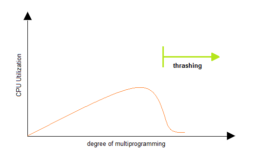
Thrashing

A process that is spending more time paging than executing is said to be thrashing. In other words it means, that the process doesn't have enough frames to hold all the pages for its execution, so it is swapping pages in and out very frequently to keep executing. Sometimes, the pages which will be required in the near future have to be swapped out.

Initially when the CPU utilization is low, the process scheduling mechanism, to increase the level of multiprogramming loads multiple processes into the memory at the same time, allocating a limited amount of frames to each process. As the memory fills up, process starts to spend a lot of time for the required pages to be swapped in, again leading to low CPU utilization because most of the proccesses are waiting for pages. Hence the scheduler loads more processes to increase CPU utilization, as this continues at a point of time the complete system comes to a stop.

To prevent thrashing we must provide processes with as many frames as they really need "right now".

Introduction to File System

A file can be "free formed", indexed or structured collection of related bytes having meaning only to the one who created it. Or in other words an entry in a directory is the file. The file may have attributes like name, creator, date, type, permissions etc.

File Structure

A file has various kinds of structure. Some of them can be :

Simple Record Structure with lines of fixed or variable lengths.
Complex Structures like formatted document or reloadable load files.
No Definite Structure like sequence of words and bytes etc.

Attributes of a File

Following are some of the attributes of a file :

Name . It is the only information which is in human-readable form.
Identifier. The file is identified by a unique tag(number) within file system.
Type. It is needed for systems that support different types of files.
Location. Pointer to file location on device.
Size. The current size of the file.
Protection. This controls and assigns the power of reading, writing, executing.
Time, date, and user identification. This is the data for protection, security, and usage monitoring.

File Access Methods

The way that files are accessed and read into memory is determined by Access methods. Usually a single access method is supported by systems while there are OS's that support multiple access methods.

1. Sequential Access

Data is accessed one record right after another is an order.
Read command cause a pointer to be moved ahead by one.
Write command allocate space for the record and move the pointer to the new End Of File.
Such a method is reasonable for tape.

2. Direct Access

This method is useful for disks.
The file is viewed as a numbered sequence of blocks or records.
There are no restrictions on which blocks are read/written, it can be dobe in any order.
User now says "read n" rather than "read next".
"n" is a number relative to the beginning of file, not relative to an absolute physical disk location.

3. Indexed Sequential Access

It is built on top of Sequential access.
It uses an Index to control the pointer while accessing files.

What is a Directory?

Information about files is maintained by Directories. A directory can contain multiple files. It can even have directories inside of them. In Windows we also call these directories as folders.

Following is the information maintained in a directory :

Name : The name visible to user.
Type : Type of the directory.
Location : Device and location on the device where the file header is located.
Size : Number of bytes/words/blocks in the file.
Position : Current next-read/next-write pointers.
Protection : Access control on read/write/execute/delete.
Usage : Time of creation, access, modification etc.
Mounting : When the root of one file system is "grafted" into the existing tree of another file system its called Mounting.

What is Banker's Algorithm?

Banker's algorithm is a deadlock avoidance algorithm. It is named so because this algorithm is used in banking systems to determine whether a loan can be granted or not.

Consider there are n account holders in a bank and the sum of the money in all of their accounts is S. Everytime a loan has to be granted by the bank, it subtracts the loan amount from the total money the bank has. Then it checks if that difference is greater than S. It is done because, only then, the bank would have enough money even if all the n account holders draw all their money at once.

Banker's algorithm works in a similar way in computers.

Whenever a new process is created, it must specify the maximum instances of each resource type that it needs, exactly.

Let us assume that there are n processes and m resource types. Some data structures that are used to implement the banker's algorithm are:

1. `Available`

It is an array of length m. It represents the number of available resources of each type. If Available[j] = k, then there are k instances available, of resource type R(j).

2. `Max`

It is an n x m matrix which represents the maximum number of instances of each resource that a process can request. If Max[i][j] = k, then the process P(i) can request atmost k instances of resource type R(j).

3. `Allocation`

It is an n x m matrix which represents the number of resources of each type currently allocated to each process. If Allocation[i][j] = k, then process P(i) is currently allocated k instances of resource type R(j).

4. `Need`

It is an n x m matrix which indicates the remaining resource needs of each process. If Need[i][j] = k, then process P(i) may need k more instances of resource type R(j) to complete its task.

Need[i][j] = Max[i][j] - Allocation [i][j]

Resource Request Algorithm

This describes the behavior of the system when a process makes a resource request in the form of a request matrix. The steps are:

If number of requested instances of each resource is less than the need (which was declared previously by the process), go to step 2.
If number of requested instances of each resource type is less than the available resources of each type, go to step 3. If not, the process has to wait because sufficient resources are not available yet.
Now, assume that the resources have been allocated. Accordingly do,

Available = Available - Requesti
Allocation(i) = Allocation(i) + Request(i)
Need(i) = Need(i) - Request(i)

This step is done because the system needs to assume that resources have been allocated. So there will be less resources available after allocation. The number of allocated instances will increase. The need of the resources by the process will reduce. That's what is represented by the above three operations.

After completing the above three steps, check if the system is in safe state by applying the safety algorithm. If it is in safe state, proceed to allocate the requested resources. Else, the process has to wait longer.

Safety Algorithm

Let Work and Finish be vectors of length m and n, respectively. Initially,
```
Work = Available
Finish[i] =false for i = 0, 1, ... , n - 1.
```
This means, initially, no process has finished and the number of available resources is represented by the Available array.
Find an index i such that both
```
Finish[i] ==false
Needi <= Work
```
If there is no such i present, then proceed to step 4.

It means, we need to find an unfinished process whose need can be satisfied by the available resources. If no such process exists, just go to step 4.
Perform the following:
```
Work = Work + Allocation;
Finish[i] = true;
```
Go to step 2.

When an unfinished process is found, then the resources are allocated and the process is marked finished. And then, the loop is repeated to check the same for all other processes.
If Finish[i] == true for all i, then the system is in a safe state.
That means if all processes are finished, then the system is in safe state.

Bounded Buffer Problem

Bounded buffer problem, which is also called producer consumer problem, is one of the classic problems of synchronization. Let's start by understanding the problem here, before moving on to the solution and program code.

What is the Problem Statement?

There is a buffer of n slots and each slot is capable of storing one unit of data. There are two processes running, namely, producer and consumer, which are operating on the buffer.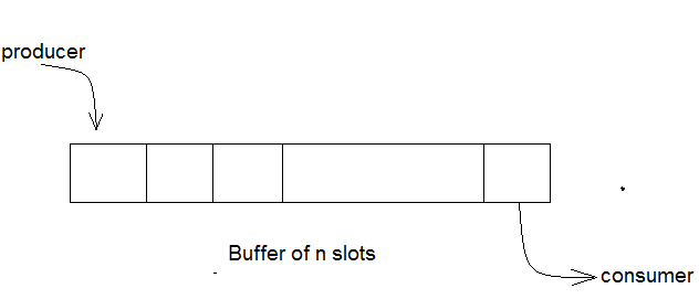

Bounded Buffer Problem

A producer tries to insert data into an empty slot of the buffer. A consumer tries to remove data from a filled slot in the buffer. As you might have guessed by now, those two processes won't produce the expected output if they are being executed concurrently.

There needs to be a way to make the producer and consumer work in an independent manner.

Here's a Solution

One solution of this problem is to use semaphores. The semaphores which will be used here are:

m, a binary semaphore which is used to acquire and release the lock.
empty, a counting semaphore whose initial value is the number of slots in the buffer, since, initially all slots are empty.
full, a counting semaphore whose initial value is 0.

At any instant, the current value of empty represents the number of empty slots in the buffer and full represents the number of occupied slots in the buffer.

The Producer Operation

The pseudocode of the producer function looks like this:

do 
{
    // wait until empty > 0 and then decrement 'empty'
    wait(empty);   
    // acquire lock
    wait(mutex);  
    
    /* perform the insert operation in a slot */
    
    // release lock
    signal(mutex);  
    // increment 'full'
    signal(full);   
} 
while(TRUE)

Looking at the above code for a producer, we can see that a producer first waits until there is atleast one empty slot.
Then it decrements the empty semaphore because, there will now be one less empty slot, since the producer is going to insert data in one of those slots.
Then, it acquires lock on the buffer, so that the consumer cannot access the buffer until producer completes its operation.
After performing the insert operation, the lock is released and the value of full is incremented because the producer has just filled a slot in the buffer.

The Consumer Operation

The pseudocode for the consumer function looks like this:

do 
{
    // wait until full > 0 and then decrement 'full'
    wait(full);
    // acquire the lock
    wait(mutex);  
    
    /* perform the remove operation in a slot */ 
    
    // release the lock
    signal(mutex); 
    // increment 'empty'
    signal(empty); 
} 
while(TRUE);

The consumer waits until there is atleast one full slot in the buffer.
Then it decrements the full semaphore because the number of occupied slots will be decreased by one, after the consumer completes its operation.
After that, the consumer acquires lock on the buffer.
Following that, the consumer completes the removal operation so that the data from one of the full slots is removed.
Then, the consumer releases the lock.
Finally, the empty semaphore is incremented by 1, because the consumer has just removed data from an occupied slot, thus making it empty.

Dining Philosophers Problem

The dining philosophers problem is another classic synchronization problem which is used to evaluate situations where there is a need of allocating multiple resources to multiple processes.

What is the Problem Statement?

Consider there are five philosophers sitting around a circular dining table. The dining table has five chopsticks and a bowl of rice in the middle as shown in the below figure.

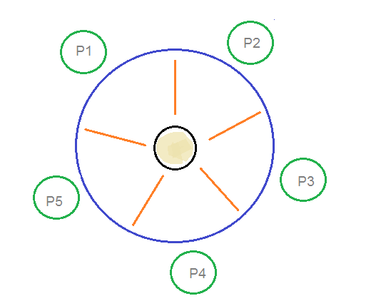
Dining Philosophers Problem

At any instant, a philosopher is either eating or thinking. When a philosopher wants to eat, he uses two chopsticks - one from their left and one from their right. When a philosopher wants to think, he keeps down both chopsticks at their original place.

Here's the Solution

From the problem statement, it is clear that a philosopher can think for an indefinite amount of time. But when a philosopher starts eating, he has to stop at some point of time. The philosopher is in an endless cycle of thinking and eating.

An array of five semaphores, stick[5], for each of the five chopsticks.

The code for each philosopher looks like:

while(TRUE) 
{
    wait(stick[i]);
    /* 
        mod is used because if i=5, next 
        chopstick is 1 (dining table is circular)
    */
    wait(stick[(i+1) % 5]);  
                    
    /* eat */
    signal(stick[i]);
    
    signal(stick[(i+1) % 5]); 
    /* think */
}

When a philosopher wants to eat the rice, he will wait for the chopstick at his left and picks up that chopstick. Then he waits for the right chopstick to be available, and then picks it too. After eating, he puts both the chopsticks down.

But if all five philosophers are hungry simultaneously, and each of them pickup one chopstick, then a deadlock situation occurs because they will be waiting for another chopstick forever. The possible solutions for this are:

A philosopher must be allowed to pick up the chopsticks only if both the left and right chopsticks are available.
Allow only four philosophers to sit at the table. That way, if all the four philosophers pick up four chopsticks, there will be one chopstick left on the table. So, one philosopher can start eating and eventually, two chopsticks will be available. In this way, deadlocks can be avoided.

What is Readers Writer Problem?

Readers writer problem is another example of a classic synchronization problem. There are many variants of this problem, one of which is examined below.

The Problem Statement

There is a shared resource which should be accessed by multiple processes. There are two types of processes in this context. They are reader and writer. Any number of readers can read from the shared resource simultaneously, but only one writer can write to the shared resource. When a writeris writing data to the resource, no other process can access the resource. A writer cannot write to the resource if there are non zero number of readers accessing the resource at that time.

The Solution

From the above problem statement, it is evident that readers have higher priority than writer. If a writer wants to write to the resource, it must wait until there are no readers currently accessing that resource.

Here, we use one mutex m and a semaphore w. An integer variable read_count is used to maintain the number of readers currently accessing the resource. The variable read_count is initialized to 0. A value of 1 is given initially to m and w.

Instead of having the process to acquire lock on the shared resource, we use the mutex m to make the process to acquire and release lock whenever it is updating the read_count variable.

The code for the writer process looks like this:

while(TRUE) 
{
    wait(w);
    
   /* perform the write operation */
   
   signal(w);
}

And, the code for the reader process looks like this:

while(TRUE) 
{
    //acquire lock
    wait(m);
    read_count++;
    if(read_count == 1)
        wait(w);
    
    //release lock  
    signal(m);  
    
    /* perform the reading operation */
    
    // acquire lock
    wait(m);   
    read_count--;
    if(read_count == 0)
        signal(w);
        
    // release lock
    signal(m);  
}

Here is the Code uncoded(explained)

As seen above in the code for the writer, the writer just waits on the w semaphore until it gets a chance to write to the resource.
After performing the write operation, it increments w so that the next writer can access the resource.
On the other hand, in the code for the reader, the lock is acquired whenever the read_count is updated by a process.
When a reader wants to access the resource, first it increments the read_count value, then accesses the resource and then decrements the read_count value.
The semaphore w is used by the first reader which enters the critical section and the last reader which exits the critical section.
The reason for this is, when the first readers enters the critical section, the writer is blocked from the resource. Only new readers can access the resource now.
Similarly, when the last reader exits the critical section, it signals the writer using the w semaphore because there are zero readers now and a writer can have the chance to access the resource.

Secondary Storage and Disk Scheduling Algorithms

Secondary storage devices are those devices whose memory is non volatile, meaning, the stored data will be intact even if the system is turned off. Here are a few things worth noting about secondary storage.

Secondary storage is also called auxiliary storage.
Secondary storage is less expensive when compared to primary memory like RAMs.
The speed of the secondary storage is also lesser than that of primary storage.
Hence, the data which is less frequently accessed is kept in the secondary storage.
A few examples are magnetic disks, magnetic tapes, removable thumb drives etc.

Magnetic Disk Structure

In modern computers, most of the secondary storage is in the form of magnetic disks. Hence, knowing the structure of a magnetic disk is necessary to understand how the data in the disk is accessed by the computer.

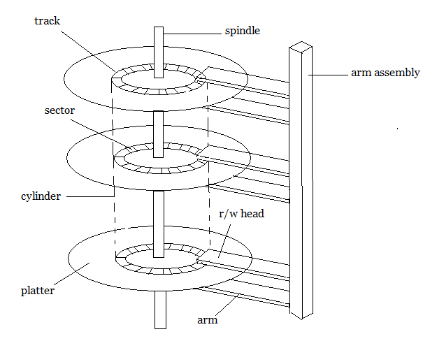
Structure of a magnetic disk

A magnetic disk contains several platters. Each platter is divided into circular shaped tracks. The length of the tracks near the centre is less than the length of the tracks farther from the centre. Each track is further divided into sectors, as shown in the figure.

Tracks of the same distance from centre form a cylinder. A read-write head is used to read data from a sector of the magnetic disk.

The speed of the disk is measured as two parts:

Transfer rate: This is the rate at which the data moves from disk to the computer.
Random access time: It is the sum of the seek time and rotational latency.

Seek time is the time taken by the arm to move to the required track. Rotational latency is defined as the time taken by the arm to reach the required sector in the track.

Even though the disk is arranged as sectors and tracks physically, the data is logically arranged and addressed as an array of blocks of fixed size. The size of a block can be 512 or 1024 bytes. Each logical block is mapped with a sector on the disk, sequentially. In this way, each sector in the disk will have a logical address.

Disk Scheduling Algorithms

On a typical multiprogramming system, there will usually be multiple disk access requests at any point of time. So those requests must be scheduled to achieve good efficiency. Disk scheduling is similar to process scheduling. Some of the disk scheduling algorithms are described below.

First Come First Serve

This algorithm performs requests in the same order asked by the system. Let's take an example where the queue has the following requests with cylinder numbers as follows:

98, 183, 37, 122, 14, 124, 65, 67

Assume the head is initially at cylinder 56. The head moves in the given order in the queue i.e., 56→98→183→...→67.

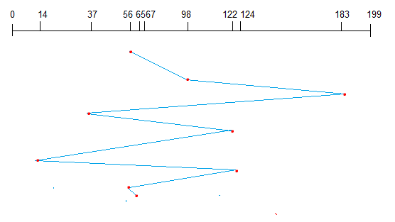
Shortest Seek Time First (SSTF)

Here the position which is closest to the current head position is chosen first. Consider the previous example where disk queue looks like,

98, 183, 37, 122, 14, 124, 65, 67

Assume the head is initially at cylinder 56. The next closest cylinder to 56 is 65, and then the next nearest one is 67, then 37, 14, so on.

SCAN algorithm

This algorithm is also called the elevator algorithm because of it's behavior. Here, first the head moves in a direction (say backward) and covers all the requests in the path. Then it moves in the opposite direction and covers the remaining requests in the path. This behavior is similar to that of an elevator. Let's take the previous example,

98, 183, 37, 122, 14, 124, 65, 67

Assume the head is initially at cylinder 56. The head moves in backward direction and accesses 37and 14. Then it goes in the opposite direction and accesses the cylinders as they come in the path.

Introduction to System Calls

To understand system calls, first one needs to understand the difference between kernel mode and user mode of a CPU. Every modern operating system supports these two modes.

Modes supported by the operating system

Kernel Mode

When CPU is in kernel mode, the code being executed can access any memory address and any hardware resource.
Hence kernel mode is a very privileged and powerful mode.
If a program crashes in kernel mode, the entire system will be halted.

User Mode

When CPU is in user mode, the programs don't have direct access to memory and hardware resources.
In user mode, if any program crashes, only that particular program is halted.
That means the system will be in a safe state even if a program in user mode crashes.
Hence, most programs in an OS run in user mode.

System Call

When a program in user mode requires access to RAM or a hardware resource, it must ask the kernel to provide access to that resource. This is done via something called a system call.

When a program makes a system call, the mode is switched from user mode to kernel mode. This is called a context switch.

Then the kernel provides the resource which the program requested. After that, another context switch happens which results in change of mode from kernel mode back to user mode.

Generally, system calls are made by the user level programs in the following situations:

Creating, opening, closing and deleting files in the file system.
Creating and managing new processes.
Creating a connection in the network, sending and receiving packets.
Requesting access to a hardware device, like a mouse or a printer.

In a typical UNIX system, there are around 300 system calls. Some of them which are important ones in this context, are described below.

Fork()

The fork() system call is used to create processes. When a process (a program in execution) makes a fork() call, an exact copy of the process is created. Now there are two processes, one being the parent process and the other being the child process.

The process which called the fork() call is the parent process and the process which is created newly is called the child process. The child process will be exactly the same as the parent. Note that the process state of the parent i.e., the address space, variables, open files etc. is copied into the child process. This means that the parent and child processes have identical but physically different address spaces. The change of values in parent process doesn't affect the child and vice versa is true too.

Both processes start execution from the next line of code i.e., the line after the fork() call. Let's look at an example:

// example.c
#include <stdio.h>
void main() 
{
    int val;  
    val = fork();   // line A
    printf("%d", val);  // line B
}

When the above example code is executed, when line A is executed, a child process is created. Now both processes start execution from line B. To differentiate between the child process and the parent process, we need to look at the value returned by the fork() call.

The difference is that, in the parent process, fork() returns a value which represents the process ID of the child process. But in the child process, fork() returns the value 0.

This means that according to the above program, the output of parent process will be the process IDof the child process and the output of the child process will be 0.

Exec()

The exec() system call is also used to create processes. But there is one big difference between fork() and exec() calls. The fork() call creates a new process while preserving the parent process. But, an exec() call replaces the address space, text segment, data segment etc. of the current process with the new process.

It means, after an exec() call, only the new process exists. The process which made the system call, wouldn't exist.

There are many flavors of exec() in UNIX, one being exec1() which is shown below as an example:

// example2.c
#include <stdio.h>
void main() 
{
    execl("/bin/ls", "ls", 0);      // line A
    printf("This text won't be printed unless an error occurs in exec().");
}

As shown above, the first parameter to the execl() function is the address of the program which needs to be executed, in this case, the address of the ls utility in UNIX. Then it is followed by the name of the program which is ls in this case and followed by optional arguments. Then the list should be terminated by a NULL pointer (0).

When the above example is executed, at line A, the ls program is called and executed and the current process is halted. Hence the printf() function is never called since the process has already been halted. The only exception to this is that, if the execl() function causes an error, then the printf()function is executed.

petek, 23. marec 2018